A small comparison of two search algorithms

For those that have been in the web development industry for a while, you know that in most cases developers use high level frameworks such as Django or Rails for their projects. These frameworks are interesting because they deal with the basic functionalities leaving us free to implement business rules and other higher level features. However, from time to time it is important for us developers to revisit the basics of Computer Science and play a bit with the simplest algorithms. Even if it takes an hour of our time, the intellectuals benefits will certainly be interesting

For this blog post, I decided to do a little comparison between two methods to find values on sorted lists: the linear-search and the binary-search algorithms. This comparison is interesting because it allows us to see the practical difference between a linear time algorithm and a logarithmic time algorithm. But it also allows us to demonstrate that theoretical knowledge is not so far removed from practice.

Linear search algorithm

The linear search is a baseline, brute-force, algorithm to find the position of a value in a sorted list. It is also a fairly simple algorithm: you start on the first position of the list and traverse all elements until you find the value you want. Here is an implementation in Python:

def linear_search(value, list):
    """
    Returns the index of a value in the list.

    """

    for index, val in enumerate(list):
        if value == val:
            return index

    return index

In a very simple and general way, all algorithms that have one for loop and do not have any tricks to exit the loop, can be considered linear time algorithms or O(n) in the Big-O notation. In a similar way, algorithms that have two for loops, being one contained in the other, are generally quadratic time algorithms, or O(n²).

Binary search algorithm

The problem of the linear search algorithm is that it doesn't care if the list is sorted or not, as it traverses all its elements until it finds the wanted value. However, smarter algorithms should do better than that. The binary search algorithm uses a kind of divide and conquer technique to exploit the sorted list in the following way:

1. Checks the number in the middle of the list.
2. If the searched number is smaller, gets the lower half of the list and goes back to step 1.
3. If the searched number is higher, gets the upper half of the list and goes back to step 1.
4. If the numbers match, done.

There are many possible implementations of the binary-search algorithm, and this is one:

def binary_search(value, list):
    """
    Return the index of a value in the list using binary search.

    """

    index = len(list) // 2

    while value != list[index]:

        if value > list[index]:
            list = list[index:]
        else:
            list = list[:index]

        index = len(list) // 2

    return index

Unfortunately, it is harder to find the theoretical behavior of these kind of algorithms. But in this specific case, since the algorithm does not traverse all the n elements of the list, its time complexity must certainly be smaller than n. In fact, in the Big-O notation, this algorithm has logarithmic complexity - O(log n).

A comparison of algorithms

To compare both methods, I made a small change to the algorithms in order to return the number of iterations that each one does until it finds the number in the list. Then, for random sorted lists of several sizes, each algorithm was executed 100 times and the average number of iterations was calculated. The source code for this comparison can be found in this gist.

The next figure shows the average number of iterations of each algorithm for lists of sizes ranging 10 to 100:

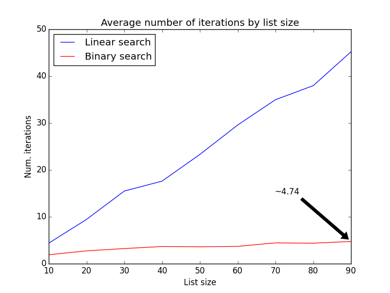
The average number of iterations grows linearly with the linear-search algorithm, while the growth is slower for the binary-search. But the difference is more noticeable when the lists grow larger:

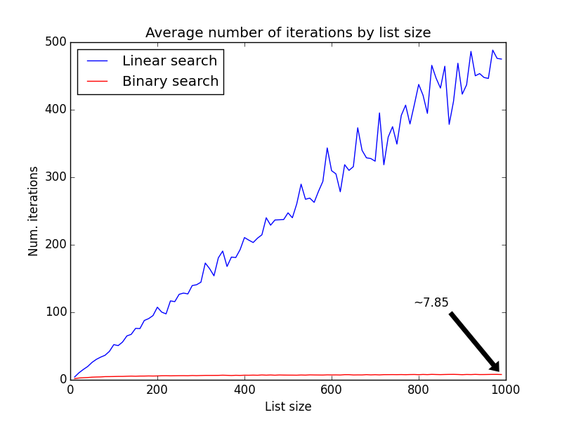
So while the linear-search algorithm does an average of 480 iterations until it finds a value in a list of size 1000, the binary-search algorithm does an average of 7.85. Interestingly, 7.85 is not far from the theoretical value for this algorithm - O(log n) => log(1000) = 6.9.

These kind of methods are so interesting that many binary-something algorithms have been invented to solve similar problems, such as the binary search trees and the B-trees. Some of the practical applications of these algorithms are in the database engines. For instance, when you do a simple query such as select * from users where email='someone@somewhere.net', databases engines will, by default, perform a linear search on the users table. We can usually increase the speed of these queries by creating indexes on the tables, which in most cases will generate data structures such as the B-tree.

In a general way, time-efficient algorithms usually exploit specific particularities on the data. The binary search method, for instance, only works on sorted data. For unsorted data, the binary search may not find the correct index at all, and only probabilistic algorithms may have a chance of beating the linear-search method (edit: I published a comparison here).

So the next time you decide to use a linear-search algorithm in a critical performance application, you'll know what you're getting into!